
This work is licensed under a Creative Commons Attribution 4.0 International License.
Analyzing PIV data of a longitudinal vortex
In this notebook, we analyze particle image velocimetry (PIV) data of a dynamically meandering longitudinal vortex. The data were recorded and provided by Nils Rathje of TU Braunschweig’s institut of fluid mechanics as part of a DFG-funded project. A delta-wing configuration with a swept angle of \(65^\circ\) was investigated in the institut’s low-speed wind tunnel (MUB) by means of a time-resolved stero-PIV. The data were recorded with a frequency of \(3kHz\) with \(7ms\) between double frames using the software package DaVis 8.4 by Lavision. A final window size decreased to \(32\times 32 px^2\) was used with \(50\%\) overlap, which corresponds to a resolution of \(\Delta x = \Delta y = 1,5mm \left( \widehat{=} 16px \right)\).
The flow conditions may be summarized as follows:
free stream velocity \(U_{\infty}=55.5 m/s\)
Reynolds number \(Re\approx 0.99\times 10^6\)
ambient temperature \(T\approx 37^\circ C\)
angle of attack \(\alpha = 8^\circ\)
The analysis is still preliminary and will be updated in future versions of flowTorch.
[1]:
import bisect
import torch as pt
import numpy as np
import matplotlib.pyplot as plt
import matplotlib as mpl
from flowtorch.data import CSVDataloader, mask_sphere
from flowtorch import DATASETS
from flowtorch.analysis import SVD

# increase resolution of plots
mpl.rcParams['figure.dpi'] = 160
Checking and accessing the available data
The data were exported from DaVis as .csv files, with one file for each snapshot. All snapshots are stored in the same folder. The CSVDataloader class has a class method from_davis to access such a data structure. The file name syntax in the sample data follows the pattern BXXXXX.dat, where XXXXX correspondes the the snapshot’s index. Therefore, we pass B as prefix argument to distinguish the index from the rest of the file name. The default suffix is .dat, but it can be
overwritten by passing a suffix argument.
[2]:
path = DATASETS["csv_aoa8_beta0_xc100_stereopiv"]
loader = CSVDataloader.from_davis(path, prefix="B")
times = loader.write_times
fields = loader.field_names[times[0]]
vertices = loader.vertices
print(f"First and last snapshot: {times[0]}/{times[-1]}")
print("Available fields: ", fields)
print(f"Available measurement points: {vertices.shape[0]}")
First and last snapshot: 00001/05000
Available fields:  ['Vx', 'Vy', 'Vz']
Available measurement points: 3741
[3]:
Vx, Vy, Vz = loader.load_snapshot(fields, times)
Flow field analysis
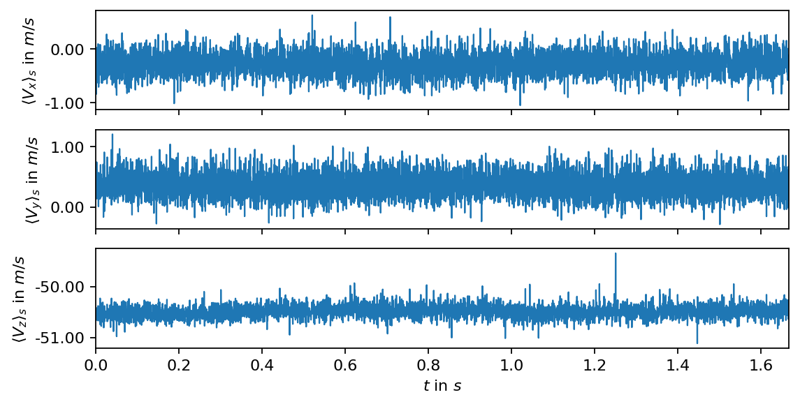
First we compute and visualize the spatial mean of each velocity component over time (the mean velocity over all measurement points in a single snapshot). The spatial average, denoted by \(\langle\rangle_s\), is an easy means to identify potential nonstationary trends or outliers in the data.
[4]:
fig, axarr = plt.subplots(3, 1, figsize=(8, 4), sharex=True)

n_times = Vx.shape[1]
freq = 3000.0
times_num = pt.linspace(0.0, n_times/freq, n_times)

labels = [r"$\langle V_{:s} \rangle_s$".format(coord) for coord in ["x", "y", "z"]]
for i, (vel, label) in enumerate(zip([Vx, Vy, Vz], labels)):
    axarr[i].plot(times_num, vel.mean(dim=0), lw=1, label=label)
    axarr[i].set_ylabel(r"{:s} in $m/s$".format(label))
    axarr[i].yaxis.set_major_formatter(mpl.ticker.FormatStrFormatter("%2.2f"))
axarr[-1].set_xlim(0, times_num[-1])
axarr[-1].set_xlabel(r"$t$ in $s$")
plt.show()
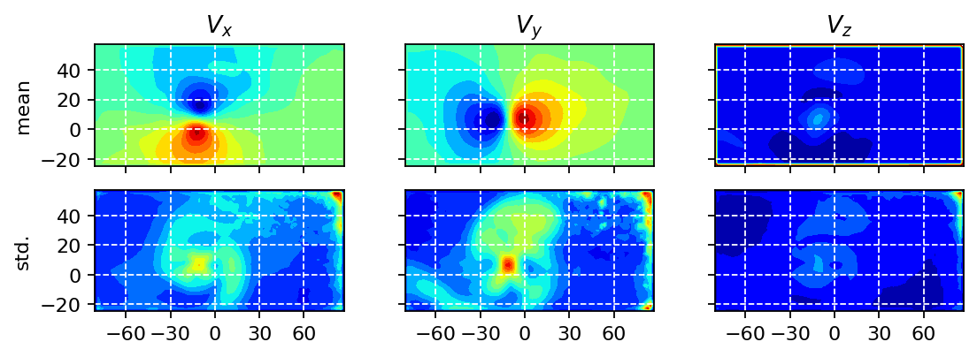
In the next step, we visualize the temporal mean and the corresponding standard deviation in each measurement point. In the resulting fields, we may be able to identify potenial outliers or areas of extreme values, e.g., close to the boundaries of the recorded images.
[5]:
fig, axarr = plt.subplots(2, 3, figsize=(8, 2.5), sharex=True, sharey=True)

axarr[0, 0].tricontourf(vertices[:, 0], vertices[:, 1], Vx.mean(dim=1), levels=15, cmap="jet")
axarr[0, 1].tricontourf(vertices[:, 0], vertices[:, 1], Vy.mean(dim=1), levels=15, cmap="jet")
axarr[0, 2].tricontourf(vertices[:, 0], vertices[:, 1], Vz.mean(dim=1), levels=15, cmap="jet")
axarr[1, 0].tricontourf(vertices[:, 0], vertices[:, 1], Vx.std(dim=1), levels=15, cmap="jet")
axarr[1, 1].tricontourf(vertices[:, 0], vertices[:, 1], Vy.std(dim=1), levels=15, cmap="jet")
axarr[1, 2].tricontourf(vertices[:, 0], vertices[:, 1], Vz.std(dim=1), levels=15, cmap="jet")

# title for each column
for ax, title in zip(axarr[0, :], [r"$V_x$", r"$V_y$", r"$V_z$"]):
    ax.set_title(title)
# label for each row
axarr[0, 0].set_ylabel("mean")
axarr[1, 0].set_ylabel("std.")
# preserve aspect ratio
for row in range(2):
    for col in range(3):
        axarr[row, col].set_aspect("equal", "box")
        axarr[row, col].xaxis.set_major_locator(plt.MaxNLocator(6))
        axarr[row, col].yaxis.set_major_locator(plt.MaxNLocator(5))
        axarr[row, col].grid(True, c="w", ls="--")
plt.show()
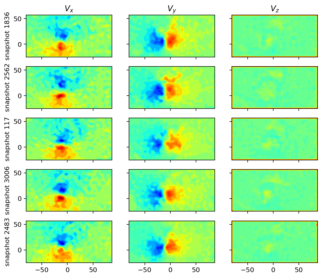
We also visualize a couple of randomly selected snapshots to have a second simple sanity check.
[6]:
n_select = 5
snapshots = np.random.choice(range(n_times), n_select)

height=1.4
fig, axarr = plt.subplots(n_select, 3, figsize=(8, height*n_select), sharex=True, sharey=True)

def color_bounds(field, factor=5):
    mean = pt.mean(field)
    std = pt.std(field)
    return {"vmin" : mean-factor*std,
            "vmax" : mean+factor*std}

for i, snap in enumerate(snapshots):
    axarr[i, 0].tricontourf(vertices[:, 0], vertices[:, 1], Vx[:, snap], levels=15, cmap="jet", **color_bounds(Vx))
    axarr[i, 1].tricontourf(vertices[:, 0], vertices[:, 1], Vy[:, snap], levels=15, cmap="jet", **color_bounds(Vy))
    axarr[i, 2].tricontourf(vertices[:, 0], vertices[:, 1], Vz[:, snap], levels=15, cmap="jet", **color_bounds(Vz))
    axarr[i, 0].set_ylabel(f"snapshot {snap}")
    for ax in axarr[i, :]:
        ax.set_aspect("equal", "box")

for ax, title in zip(axarr[0, :], [r"$V_x$", r"$V_y$", r"$V_z$"]):
    ax.set_title(title)
plt.show()
SVD analysis
Masking the data
In the visualizations above, we could observe: - spurious values (close to zero) close to the borders, which are particularly pronounced in the \(z\)-component of the velocity - a zone of spurious values in the upper right corner of the image
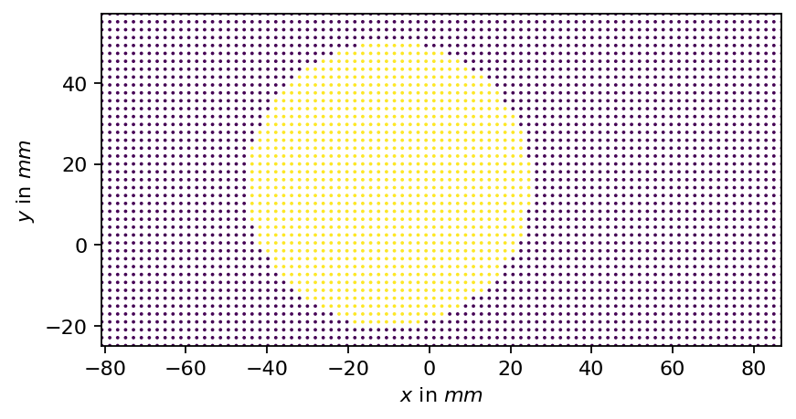
These spurious samples might compromise our analysis, which is why we create a mask to exclude the affected regions from the data. For the longitudinal vortex, a circular/spherical mask is suitable.
[7]:
mask = mask_sphere(vertices, center=[-10.0, 15], radius=35)
print(f"Selected vertices: {mask.sum().item()}/{mask.shape[0]}")
Selected vertices: 1018/3741
[8]:
fig, ax = plt.subplots()
ax.scatter(vertices[:, 0], vertices[:, 1], s=0.5, c=mask)
ax.set_aspect("equal", 'box')
ax.set_xlim(vertices[:, 0].min(), vertices[:, 0].max())
ax.set_ylim(vertices[:, 1].min(), vertices[:, 1].max())
ax.set_xlabel(r"$x$ in $mm$")
ax.set_ylabel(r"$y$ in $mm$")
plt.show()
Visualizing the SVD
In the present analysis, we are only analyzing the velocity in the main flow direction, which is the \(z\)-component.
[9]:
# allocate reduced data matrix matrix, apply the mask to the original data, and subtract the mean
selected_points = mask.sum().item()
Vz_masked = pt.zeros((selected_points, Vz.shape[1]), dtype=pt.float32)
for i in range(Vz.shape[1]):
    Vz_masked[:, i] = pt.masked_select(Vz[:, i], mask)
Vz_mean = Vz_masked.mean(dim=1).unsqueeze(-1)
Vz_masked -= Vz_mean
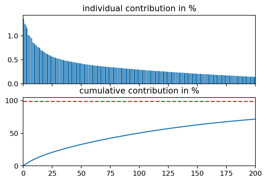
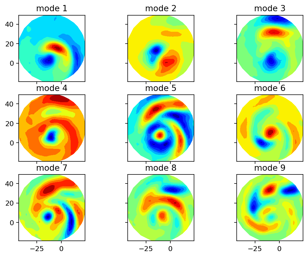
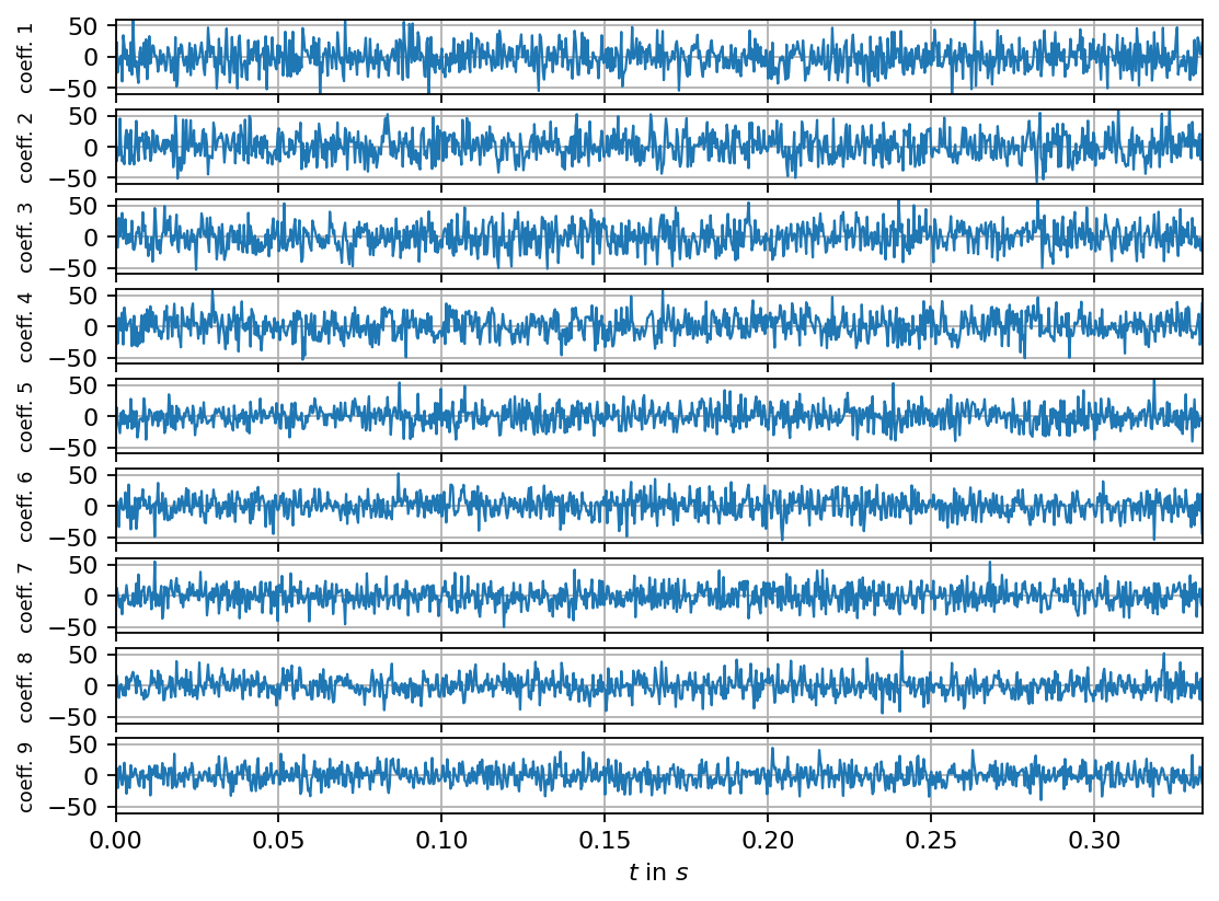
Next, we compute the singular value decomposition and visualize the singular values, the POD modes (left singular vectors) and the mode coefficients (right singular vectors multiplied by the corresponding singular value). The modes can be interpreted as coherent spatial structures while the coefficients characterize the modes’ evolution over time.
[10]:
# we set the rank to to the number of available snapshots to avoid any truncation
svd = SVD(Vz_masked, 5000)
print(svd)
SVD of a 1018x5000 data matrix
Selected/optimal rank: 5000/349
data type: torch.float32 (4b)
truncated SVD size: 23.3740Mb
[11]:
s = svd.s
s_sum = s.sum().item()
# relative contribution
s_rel = [s_i / s_sum * 100 for s_i in s]
# cumulative contribution
s_cum = [s[:n].sum().item() / s_sum * 100 for n in range(s.shape[0])]
# find out how many singular values we need to reach at least 99 percent
i_99 = bisect.bisect_right(s_cum, 99)
[12]:
fig, (ax1, ax2) = plt.subplots(2, 1, sharex=True)
ax1.bar(range(s.shape[0]), s_rel, align="edge")
ax2.plot(range(s.shape[0]), s_cum)
ax2.set_xlim(0, 200)
ax2.set_ylim(0, 105)
ax1.set_title("individual contribution in %")
ax2.set_title("cumulative contribution in %")
ax2.plot([0, i_99, i_99], [s_cum[i_99], s_cum[i_99], 0], ls="--", color="C3")
print("first {:d} singular values yield {:1.2f}%".format(i_99, s_cum[i_99]))
plt.show()
first 932 singular values yield 99.01%
[13]:
fig, axarr = plt.subplots(3, 3, figsize=(8, 6), sharex=True, sharey=True)
x = pt.masked_select(vertices[:, 0], mask)
y = pt.masked_select(vertices[:, 1], mask)
count = 0
for row in range(3):
    for col in range(3):
        axarr[row, col].tricontourf(x, y, svd.U[:, count], levels=14, cmap="jet")
        axarr[row, col].set_aspect("equal", 'box')
        # add 1 for the POD mode number since we subtracted the mean
        axarr[row, col].set_title(f"mode {count + 1}")
        count += 1
plt.show()
[14]:
n_steps = 1000
fig, axarr = plt.subplots(9, 1, figsize=(8, 6), sharex=True)
for i, ax in enumerate(axarr):
    ax.plot(times_num[:n_steps], svd.V[:n_steps, i]*svd.s[i], lw=1, label=f"coeff. mode {i+1}")
    ax.grid()
    # add 1 for the POD mode number since we subtracted the mean
    ax.set_ylabel(f"coeff. {i + 1}", fontsize=8)
    ax.set_ylim(-60, 60)

axarr[-1].set_xlabel(r"$t$ in $s$")
axarr[-1].set_xlim(times_num[0], times_num[n_steps-1])
plt.show()
[ ]: