This work is licensed under a Creative Commons Attribution 4.0 International License.

Linear algebra with PyTorch

This notebook introduces some frequently used linear Algebra and tensor operations in PyTorch. For a general introduction to important concepts of linear Algebra, refer to:

Introduction to linear Algebra by Gilbert Strang

The first version of this notebook was created by Mahdi Maktabi during his time as student assisant at TU Braunschweig’s Institute of Fluid Mechanics.

# import PyTorch and plotting libraries
import torch as pt
import visualization as vis
import matplotlib.pyplot as plt
from math import sqrt

PyTorch tensors

PyTorch provides a tensor type to define \(n\)-dimensional arrays. Each element in a tensor must be of the same type. Working with PyTorch tensors has a very similar look and feel to working with Numpy arrays. flowTorch uses PyTorch tensors as data structure for field data.

Creating tensors

# creating a vector of length 10 initialized with zeros
origin = pt.zeros(10)
origin

tensor([0., 0., 0., 0., 0., 0., 0., 0., 0., 0.])

# the two most important tensor attributes: size and dtype
print("Dimension: ", origin.size())
print("Datatype: ", origin.dtype)

Dimension:  torch.Size([10])
Datatype:  torch.float32

# create a 2D tensor with 3 rows and two columns filled with ones
ones = pt.ones((3, 2))
ones

tensor([[1., 1.],
        [1., 1.],
        [1., 1.]])

# 1D tensor with 5 linearly spaced values between zero and ten
x = pt.linspace(0, 10, 5)
x

tensor([ 0.0000,  2.5000,  5.0000,  7.5000, 10.0000])

# creating a tensor from a Python list
X_list = [
    [0, 1, 2],
    [3, 4, 5],
    [6, 7, 8],
    [9, 10, 11]
]
X = pt.tensor(X_list)
print("Created tensor of shape ", X.size())
X

Created tensor of shape  torch.Size([4, 3])

tensor([[ 0,  1,  2],
        [ 3,  4,  5],
        [ 6,  7,  8],
        [ 9, 10, 11]])

Accessing elements in a tensor

PyTorch tensors support element access via the typical square-bracket syntax. Also slicing is supported.

# accessing the element in the fourth row and thrid column
X[3, 2]

tensor(11)

# accessing the first column
X[:, 0]

tensor([0, 3, 6, 9])

# accessing the second row
X[1]

tensor([3, 4, 5])

# accessing the first two elements in the second column
X[:2, 1]

tensor([1, 4])

# accessing the last two column of the thrid row
X[2, -2:]

tensor([7, 8])

Basic tensor operations

# elementwise addition of a scalar value
# X += 2 is shorthand for X = X + 2
X = pt.zeros((2, 3))
X += 2
X

tensor([[2., 2., 2.],
        [2., 2., 2.]])

# elementwise multiplication with a scalar value
Y = X * 2
Y

tensor([[4., 4., 4.],
        [4., 4., 4.]])

# elementwise subtraction of two tensors with the same shape
X - Y

tensor([[-2., -2., -2.],
        [-2., -2., -2.]])

# elementwise multiplication of two tensors with the same shape
X * Y

tensor([[8., 8., 8.],
        [8., 8., 8.]])

# subtracting a 1D tensor from each row
ones = pt.ones((1, Y.size()[1]))
print("Shape of 1D tensor: ", ones.size())
Y - ones

Shape of 1D tensor:  torch.Size([1, 3])

tensor([[3., 3., 3.],
        [3., 3., 3.]])

# subtracting a 1D tensor from each column
twos = pt.ones((Y.size()[0]), 1) * 2
print("Shape of 1D tensor: ", twos.size())
Y - twos

Shape of 1D tensor:  torch.Size([2, 1])

tensor([[2., 2., 2.],
        [2., 2., 2.]])

# transpose (swapping rows and columns in 2D)
print("Shape of Y/Y.T: ", Y.size(), "/", Y.T.size())
Y.T

Shape of Y/Y.T:  torch.Size([2, 3]) / torch.Size([3, 2])

tensor([[4., 4.],
        [4., 4.],
        [4., 4.]])

Linear algebra with PyTorch

Scalar product

The scalar or dot product between two vectors \(\mathbf{a}\) and \(\mathbf{b}\) of length \(N\) is defined as:

\[\langle \mathbf{a}, \mathbf{b} \rangle := \sum\limits_{i=1}^{N} a_i b_i.\]

The dot product has couple of useful properties; see section 1.2 in Introduction to linear algebra.

The dot product of a vector with itself is equal to the squared length/magnitude \(\langle \mathbf{a}, \mathbf{a} \rangle = \left\|\mathbf{a}\right\|^2\)

Example:

\(\mathbf{a} = [1, 2, 2]^T\), \(\langle \mathbf{a}, \mathbf{a} \rangle = 1^2 + 2^2 + 2^2 = 9\)

a = pt.tensor([1.0, 2.0, 2.0])
len_a = pt.norm(a)

assert pt.dot(a, a) == len_a**2
pt.dot(a, a)

tensor(9.)

The cosine of the angle enclosed by two vectors of unit length is equal to their dot-product:

\[{\displaystyle \varphi =\arccos{\frac {\langle \mathbf{a} ,{\mathbf {b}\rangle}}{\left\|{\mathbf {a}}\right\|\left\|{\mathbf {b}}\right\|}}}\]

Example:

\(\mathbf {a} = [1,1,1]^T,\ \mathbf {b} = [4,2,2]^T\)

\(\left\|{\mathbf {a}}\right\| = {\sqrt {{{1}^2}+{{1}^2}+{{1}^2}}} = 1.7321\),

\(\left\|{\mathbf {b}}\right\| = {\sqrt {{{4}^2}+{{2}^2}+{{2}^2}}} = 4.8990\),

\(\langle \mathbf{a}, \mathbf{b} \rangle = 1\cdot 4+1\cdot 2+1\cdot 2 = 8\)

\({\displaystyle \varphi =\arccos {\frac {8}{1.7321\cdot 4.8990}=0.3398}}\)

a = pt.tensor([1.0, 1.0, 1.0])
b = pt.tensor([4.0, 2.0, 2.0])
c = pt.dot(a, b)/(pt.norm(a)*pt.norm(b))
angle = pt.acos(c) # angle in radians

assert pt.isclose(angle, pt.tensor(0.3398), atol=1.0E-3)
angle

tensor(0.3398)

To find a unit vector with the same direction as a given vector, we divide by the vector’s magnitude:

\[{\displaystyle \mathbf{u} = {\frac { \mathbf{a} }{\left\|{\mathbf {a}}\right\|}}}\]

Example:

\(\mathbf{a} = [3,6,1]^T\), \(\left\|{\mathbf{a}}\right\| = \sqrt {46}\)

\(\left\|{\mathbf {u}}\right\|\) = \({\sqrt {(\frac {3}{\sqrt {46}})^{2}+(\frac {6}{\sqrt {46} })^{2}+(\frac {1}{\sqrt {46} })^{2}}}=1\)

# using the div-function is equivalent to elementwise division of a tensor by a scalar in this example
# e.g., b = a / pt.norm(a) yields the same result
a = pt.tensor([3.0, 6.0, 1.0])
b = pt.div(a, pt.norm(a))
a_length = pt.norm(b)

assert pt.isclose(a_length, pt.tensor(1.0), atol=1.0E-3)
a_length

tensor(1.0000)

Two vectors are orthogonal if their dot product is zero.

Example:

\(\mathbf{a}=[3, 0]^T\), \(\mathbf{b}=[0, 2]^T\)

\({\displaystyle \varphi =\arccos {\frac {{3\cdot 0 + 0\cdot 2}}{\sqrt {2}\cdot{\sqrt {3}}}=90^{\circ} }}\)

a = pt.tensor([3.0, 0.0])
b = pt.tensor([0.0, 2.0])
c = pt.dot(a, b)/(pt.norm(a)*pt.norm(b))
d = pt.acos(c)
angle = pt.rad2deg(d)

assert pt.isclose(angle, pt.tensor(90.), atol=1.0E-4)
angle

tensor(90.)

Cross product

The cross product between two three-dimensional vectors \(\mathbf{a}\) and \(\mathbf{b}\) is defined as:

\[\mathbf{a}\times\mathbf{b} = \sum\limits_{i,j,k=1}^{3} a_i b_j \epsilon_{ijk} \mathbf{e}_k,\]

where \(\epsilon_{ijk}\) is the Levi-Civita symbol, and \(\mathbf{e}_k\) is the \(k\)-th unit vector.

Example:

\(\mathbf{a}=[1, 2, 3]^T\), \(\mathbf{b}=[3, 2, 1]^T\)

\({\mathbf{a}}\times{\mathbf{b}}=\begin{bmatrix}1 \\ 2 \\ 3 \end{bmatrix}\times\begin{bmatrix}3 \\ 2 \\ 1 \end{bmatrix}=\begin{bmatrix}2\cdot1 - 3\cdot2 \\3\cdot3 - 1\cdot1 \\1\cdot2 - 2\cdot3\end{bmatrix}\,=\begin{bmatrix}-4 \\ 8 \\ -4\end{bmatrix}\)

a = pt.tensor([1.0, 2.0, 3.0])
b = pt.tensor([3.0, 2.0, 1.0])
c = pt.cross(a, b)

assert pt.equal(c, pt.tensor([-4., 8., -4.]))
c

tensor([-4.,  8., -4.])

The cross product may be used to compute the angle between two vectors:

\[{\displaystyle \varphi =\arcsin {\frac {\left\| \mathbf{a} \times \mathbf {b}\right\|}{ \left\|{\mathbf {a}}\right\| \left\|{\mathbf {b}}\right\|}}}\]

Example:

\(\mathbf {a} = [1,-2,3]^T,\mathbf{b} = [-4,5,6]^T\)

\(\left\|{\mathbf {a}}\right\|= {\sqrt {{{1}^2}+{{-2}^2}+{{3}^2}}} = \sqrt {14}\), \(\left\|{\mathbf {b}}\right\|= {\sqrt {{{-4}^2}+{{5}^2}+{{6}^2}}} = \sqrt {77}\)

\({\displaystyle \left\|\mathbf {a\times b}\right\| ={\begin{vmatrix} \mathbf i& \mathbf j& \mathbf k \\1&-2&3\\-4&5&6\\\end{vmatrix}}}\) \({\displaystyle {\begin{aligned} =(-27)\mathbf {i} -(18)\mathbf {j} +(-3)\mathbf {k}={\sqrt {{{(-27)}^2}+{{(-18)}^2}+{{(-3)}^2}}=3{\sqrt{118}}}\end{aligned}}}\)

\({ \varphi =\arccos {\frac {3\sqrt{118}}{\sqrt {14}\sqrt {77}}=83.0023^\circ}}\)

a = pt.tensor([1.0, -2.0, 3.0])
b = pt.tensor([-4.0, 5.0, 6.0])
c = pt.norm(pt.cross(a, b))/(pt.norm(a)*pt.norm(b))
angle = pt.rad2deg(pt.asin(c))

assert pt.isclose(angle, pt.tensor(83.0023), atol=1.0E-4)
angle

tensor(83.0023)

The magnitude of the cross product yields the area of the parallelogram spanned by two vectors \(\mathbf {a}\) and \(\mathbf {b}\).

\[A = {\displaystyle \left\|\mathbf {a} \times \mathbf {b} \right\|=\left\|\mathbf {a} \right\|\left\|\mathbf {b} \right\| \sin \varphi .}\]

Example:

\(\mathbf {a} = [1,1,1]^T\), \(\mathbf {b} = [1,1,2]^T\)

\(\mathbf{c}=\mathbf{a}\times\mathbf{b} = [1, -1, 0]^T\), \(\left\|\mathbf{c}\right\|=\sqrt{2}\)

a = pt.tensor([1.0, 1.0, 1.0])
b = pt.tensor([1.0, 1.0, 2.0])
c_mag = pt.norm(pt.cross(a, b))

assert pt.isclose(c_mag, pt.tensor(1.4142), atol=1.0E-4)
c_mag

tensor(1.4142)

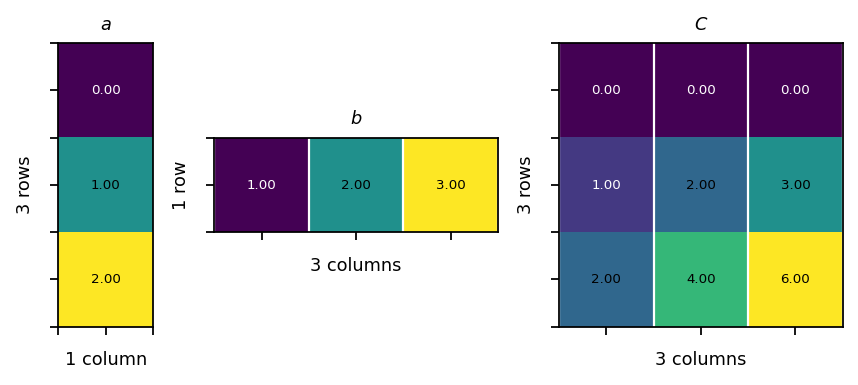
Outer product

The outer product of two vectors is a matrix. If the two vectors have dimensions \(m\) and \(n\), their outer product is an \(m\times n\) matrix. Consider the vectors \(\mathbf{a}=[a_{1},a_{2},\dots ,a_{m}]^T\) and \(\mathbf{b} =[b_{1},b_{2},\dots ,b_{n}]^T\). Their outer product, denoted by \(\mathbf{a}\otimes \mathbf{b}\), is obtained by multiplying each element of \(\mathbf{a}\) with each element of \(\mathbf{b}\) as follows:

\[\begin{split}\mathbf{C} = \mathbf {a} \otimes \mathbf {b} ={\begin{bmatrix}a_{1}b_{1}&a_{1}b_{2}&\dots &a_{1}b_{n}\\a_{2}b_{1}&a_{2}b_{2}&\dots &a_{2}b_{n}\\\vdots &\vdots &\ddots &\vdots \\a_{m}b_{1}&a_{m}b_{2}&\dots &a_{m}b_{n}\end{bmatrix}}\end{split}\]

Example:

\(\begin{bmatrix}0 \\ 1 \\ 2 \end{bmatrix}\begin{bmatrix}1&2&3 \end{bmatrix}=\begin{bmatrix}0&0&0\\1&2&3 \\2&4&6\end{bmatrix}\)

a = pt.tensor([[0, 1, 2]]).view(3, 1)
b = pt.tensor([1, 2, 3]).view(1, 3)
C = pt.mm(a, b)

assert pt.equal(C, pt.tensor([[0, 0, 0],[1, 2, 3],[2, 4, 6]]))
vis.plot_matrices_as_heatmap([a, b, C], [r"$a$", r"$b$", r"$C$"])

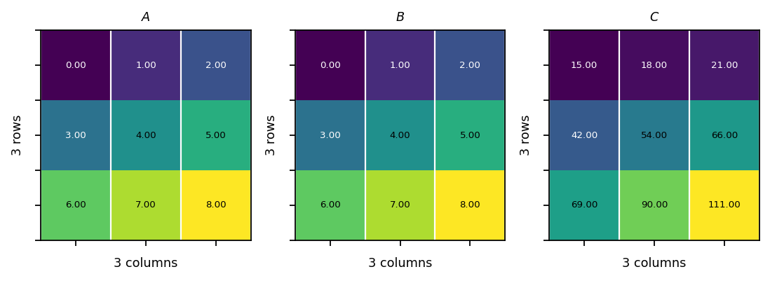
Matrix multiplication

The product of two matrices \(\mathbf{C} = \mathbf{AB}\) creates a new matrix with the same number of rows as \(\mathbf{A}\) and the same number of columns as \(\mathbf{B}\). The number of columns of matrix \(\mathbf{A}\) must be equal to the number of row of matrix \(\mathbf{B}\).

\[\begin{split}{\begin{bmatrix}c_{11}&c_{12}&\cdots &c_{1p}\\c_{21}&c_{22}&\cdots &c_{2p}\\\vdots &\vdots &\ddots &\vdots \\c_{m1}&c_{m2}&\cdots &c_{mp}\\\end{bmatrix}}= {\begin{bmatrix}a_{11}&a_{12}&\cdots &a_{1n}\\a_{21}&a_{22}&\cdots &a_{2n}\\\vdots &\vdots &\ddots &\vdots \\a_{m1}&a_{m2}&\cdots &a_{mn}\\\end{bmatrix}}{\begin{bmatrix}b_{11}&b_{12}&\cdots &b_{1p}\\b_{21}&b_{22}&\cdots &b_{2p}\\\vdots &\vdots &\ddots &\vdots \\b_{n1}&b_{n2}&\cdots &b_{np}\\\end{bmatrix}}\end{split}\]

The coeffients of the resulting matrix are computed as follows:

\[c_{ij}=a_{i1}b_{1j}+a_{i2}b_{2j}+\cdots +a_{ik}b_{kj}=\sum _{k=1}^{n}a_{ik}b_{kj}\]

Example:

\[\begin{split}{\mathbf{A}}{\mathbf{B}}=\begin{bmatrix}0&1&2 \\ 3&4&5 \\ 6&7&8 \end{bmatrix}\begin{bmatrix}0&1&2 \\ 3&4&5 \\ 6&7&8 \end{bmatrix}=\begin{bmatrix}15&18&21\\42&54&66 \\69&90&111 \end{bmatrix}\end{split}\]

A = pt.tensor(
    [[0, 1, 2],
     [3, 4, 5],
     [6, 7, 8]]
)
B = pt.tensor(
    [[0, 1, 2],
     [3, 4, 5],
     [6, 7, 8]]
)
C = pt.mm(A, B)

assert pt.equal(C, pt.tensor([[15, 18, 21],[42, 54, 66],[69, 90, 111]]))
vis.plot_matrices_as_heatmap([A, B, C], [r"$A$", r"$B$", r"$C$"])

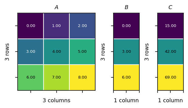
Example 2:

\({\mathbf{A}}{\mathbf{B}}=\begin{bmatrix}0&1&2 \\ 3&4&5 \\ 6&7&8 \end{bmatrix}\begin{bmatrix}0 \\ 3 \\ 6 \end{bmatrix}=\begin{bmatrix}15\\14\\23 \end{bmatrix}\)

A = pt.tensor(
    [[0., 1., 2.],
     [3., 4., 5.],
     [6., 7., 8.]]
)
B = pt.tensor([[0., 3., 6.]]).view(3, 1)
C = pt.mm(A, B)

# instead of the mm function we can also use the @ opertaor
assert pt.equal(C, A @ B)
assert pt.equal(C, pt.tensor([15., 42., 69.]).view(3, 1))
vis.plot_matrices_as_heatmap([A, B, C], [r"$A$", r"$B$", r"$C$"])

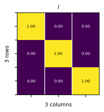
Identity matrix

The identity matrix is a square matrix with a value of one on the diagonal and zero elsewhere.

\[\begin{split}I={\begin{bmatrix}1&0&0&\cdots &0\\0&1&0&\cdots &0\\0&0&1&\cdots &0\\\vdots &\vdots &\vdots &\ddots &\vdots \\0&0&0&\cdots &1\end{bmatrix}}\end{split}\]

ones = pt.ones(3)
identity = pt.diag(ones)

assert pt.allclose(pt.eye(3), identity)
vis.plot_matrices_as_heatmap([identity], [r"$I$"])

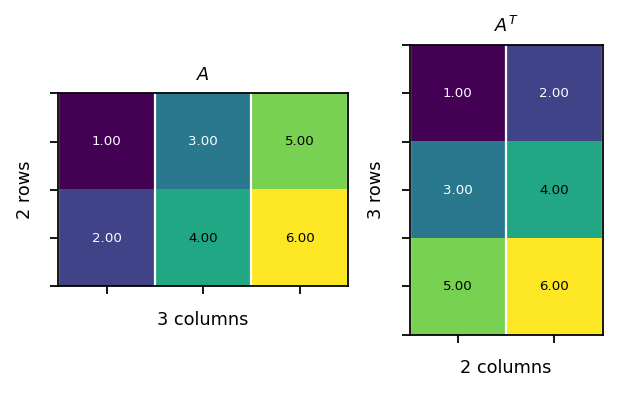
Transpose of a matrix

The transpose of a matrix is obtained by swaping its rows and columns.

\[\begin{split}\mathbf{A}= \begin{bmatrix} a_{11} & \dots & a_{1n} \\ \vdots & & \vdots \\ a_{m1} & \dots & a_{mn} \end{bmatrix},\quad \mathbf{A}^T= \begin{bmatrix} a_{11} & \dots & a_{m1} \\ \vdots & & \vdots \\ a_{1n} & \dots & a_{mn} \end{bmatrix}\end{split}\]

Example:

\(\begin{bmatrix}1&3&5\\2&4&6\end{bmatrix}^T=\begin{bmatrix}1&2\\3&4\\5&6\end{bmatrix}\)

A = pt.tensor(
    [[1, 3, 5],
     [2, 4, 6]]
)
AT = pt.tensor(
    [[1, 2],
     [3, 4],
     [5, 6]]
)

assert (A.T - AT).sum().item() == 0
vis.plot_matrices_as_heatmap([A, A.T], [r"$A$", r"$A^T$"])

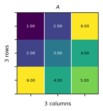
Symmetric matrix

A symmetric matrix is a square matrix that is equal to its transpose: \(\mathbf{A} = \mathbf{A}^T\). The matrix coefficients are symmetric with respect to the diagonal.

Example:

\({\begin{bmatrix}1&2&6\\2&3&4\\6&4&5\end{bmatrix}}\)

A = pt.tensor(
    [[1, 2, 6],
     [2, 3, 4],
     [6, 4, 5]]
)
AT = pt.transpose(A, 0, 1)

assert pt.equal(A, AT)
vis.plot_matrices_as_heatmap([A], [r"$A$"])

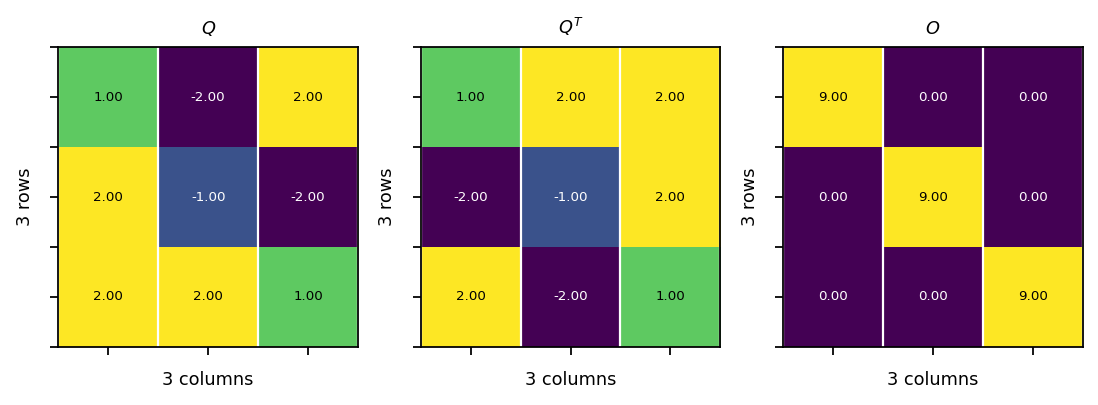
Orthogonal matrix

A matrix is orthogonal if its column vectors form an orthogonal basis. The column vectors are orthogonal if:

\[\begin{split}\langle\mathbf{q}_i, \mathbf{q}_j\rangle= \begin{cases} 0 & \text{if} ~i\neq j \\ \neq 0 & \text{if}~i=j \end{cases}\end{split}\]

Example:

\({\mathbf{Q}}{\mathbf{Q^{T}}}=\begin{bmatrix}1&-2&2 \\ 2&-1&-2 \\ 2&2&1 \end{bmatrix}\begin{bmatrix} 1&2&2 \\ -2&-1&2 \\ 2&-2&1 \end{bmatrix}=\begin{bmatrix}9&0&0\\0&9&0 \\0&0&9 \end{bmatrix}\)

Q = pt.tensor(
    [[1.0, -2.0,  2.0],
     [2.0, -1.0, -2.0],
     [2.0,  2.0,  1.0]]
)
QT = pt.transpose(Q, 0, 1)
O = pt.mm(Q, QT)

assert pt.allclose(pt.eye(3)*9, O)
vis.plot_matrices_as_heatmap([Q, QT, O], [r"$Q$", r"$Q^T$", r"$O$"])

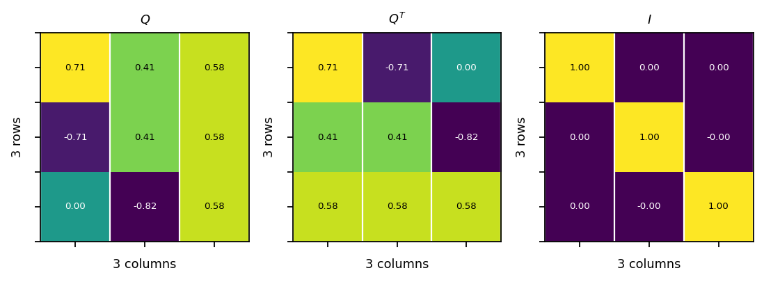
Orthonormal matrix

The vectors \(\mathbf{q}_i\) are orthonormal if:

\[\begin{split}\langle\mathbf{q}_i, \mathbf{q}_j\rangle={\begin{cases}0&{\text{if}}~i\neq j\quad\text{(orthogonal vectors)} \\1&{\text{if}~i=j\quad\text{(unit vectors: $|\mathbf{q}_i|$ = 1)}}\end{cases}}\end{split}\]

A matrix \(\mathbf{Q}\) with orthonormal column vectors satisfies the relation \(\mathbf{Q}^T\mathbf{Q} = \mathbf{Q}\mathbf{Q}^T = \mathbf{I}\).

Example:

\({\mathbf{Q}^T}{\mathbf{Q}}=\begin{bmatrix}{\frac {1}{\sqrt{2}}}&{\frac {1}{\sqrt{6}}}&{\frac {1}{\sqrt{3}}}\\{\frac {-1}{\sqrt{2}}}&{\frac {1}{\sqrt{6}}}&{\frac {1}{\sqrt{3}}}\\0&{\frac {-2}{\sqrt{6}}}&{\frac {1}{\sqrt{3}}}\end{bmatrix}\begin{bmatrix}{\frac {1}{\sqrt{2}}}&{\frac {-1}{\sqrt{2}}}&0\\{\frac {1}{\sqrt{6}}}&{\frac {1}{\sqrt{6}}}&{\frac {-2}{\sqrt{6}}}\\{\frac {1}{\sqrt{3}}}&{\frac {1}{\sqrt{3}}}&{\frac {1}{\sqrt{3}}}\end{bmatrix}=\begin{bmatrix}1&0&0\\0&1&0 \\0&0&1 \end{bmatrix}\)

Q = pt.tensor(
    [[1./sqrt(2), 1./sqrt(6), 1./sqrt(3)],
     [-1./sqrt(2), 1./sqrt(6), 1./sqrt(3)],
     [0./sqrt(2), -2./sqrt(6), 1./sqrt(3)]]
)
QT = pt.transpose(Q, 0, 1)
I = pt.mm(QT, Q)

assert pt.allclose(pt.eye(3), I, atol=1.0E-6)
assert pt.allclose(pt.mm(Q, QT), pt.mm(QT, Q), atol=1.0E-6)
vis.plot_matrices_as_heatmap([Q, QT, I], [r"$Q$", r"$Q^T$", r"$I$"])

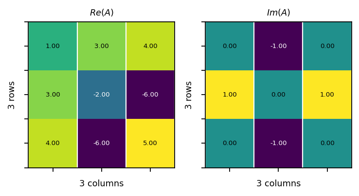
Hermitian matrix

A Hermitian matrix is a complex matrix that is equal to its conjugate transpose:

\[\mathbf{A}=\overline{\mathbf{A}}^T\]

Example:

\({\mathbf{A} = \begin{bmatrix}1&3-{\mathrm {j}}&4\\3+{\mathrm {j}}&-2&-6+{\mathrm {j}}\\4&-6-{\mathrm {j}}&5\end{bmatrix},} \quad {\overline{\mathbf{A}} = \begin{bmatrix}1&3+{\mathrm {j}}&4\\3-{\mathrm {j}}&-2&-6-{\mathrm {j}}\\4&-6+{\mathrm {j}}&5\end{bmatrix}}\)

\({\mathbf{A}=\overline{\mathbf{A}}^T= \begin{bmatrix}1&3-{\mathrm {j}}&4\\3+{\mathrm {j}}&-2&-6+{\mathrm {j}}\\4&-6-{\mathrm {j}}&5\end{bmatrix}}\)

A = pt.tensor(
    [[1., 3.-1j , 4.],
     [3.+1j, -2., -6.+1j],
     [4., -6.-1j, 5.]]
)
AH = A.conj().T

assert pt.allclose(A, AH)
vis.plot_matrices_as_heatmap([A.real, A.imag], [r"$Re(A)$", r"$Im(A)$"])

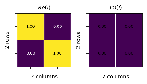
Unitary matrix

A unitary matrix is a complex square matrix whose column vectors form an orthonormal basis. The matrix product of a unitary matrix with its conjugate transpose, denoted by \(\dagger\), yields the identity matrix:

\[\mathbf{Q}\mathbf{Q}^\dagger = \mathbf{I}\]

Example:

\({\mathbf{Q}={\frac {1}{2}}\begin{bmatrix}1+i&1-i\\1-i&1+i\end{bmatrix}},\quad {\mathbf{Q}\mathbf{Q}^\dagger={\frac {1}{4}}\begin{bmatrix}1+i&1-i\\1-i&1+i\end{bmatrix}}{\begin{bmatrix}1-i&1+i\\1+i&1-i\end{bmatrix}}=\begin{bmatrix}1&0\\0&1 \end{bmatrix}= \mathbf{I}\)

Q = pt.tensor(
    [[(1+1j)/2.0, (1-1j)/2.0],
     [(1-1j)/2.0, (1+1j)/2.0]]
)
QH = pt.conj(Q).T
I = pt.mm(Q, QH)

assert pt.allclose(I, pt.eye(2, dtype=pt.cfloat))
assert pt.allclose(I, pt.mm(QH, Q))
vis.plot_matrices_as_heatmap([I.real, I.imag], [r"$Re(I)$", r"$Im(I)$"])

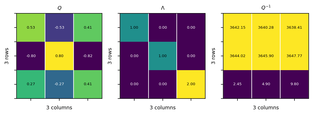
Matrix decompositions

Eigen-decomposition

The eigen-decomposition of a square matrix \(\mathbf{A}\) is:

\[\mathbf{A}=\mathbf{Q}\mathbf{\Lambda}\mathbf{Q}^{-1}\]

\(\mathbf{Q}\) is a square matrix formed by the eigenvecctors of \(\mathbf{A}\), and \(\mathbf{\Lambda}\) is a diagonal matrix whose diagonal elements are the corresponding eigenvalues.

A = pt.tensor(
    [[0.0, 0.0,  2.0],
     [1.0, 0.0, -5.0],
     [0.0, 1.0,  4.0]]
)

# the eigen decomposition returns complex tensors; to compare them with
# the original tensor, we remove the imaginary part
val, vec = pt.linalg.eig(A)
Q = vec.real
L = pt.diag(val).real
invQ = pt.linalg.inv(Q)

assert pt.allclose(pt.mm(Q, invQ), pt.eye(3), atol=1.0E-3)
assert pt.allclose(A, pt.mm(Q, L).mm(invQ), atol=1.0E-2)
vis.plot_matrices_as_heatmap([Q, L, invQ], [r"$Q$", r"$\Lambda$", r"$Q^{-1}$"])

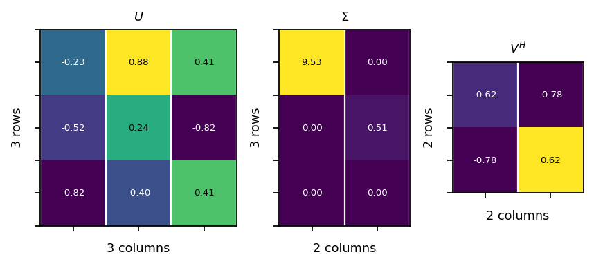
Singular value decomposition (SVD)

The SVD is a factorization of a real or complex matrix that generalizes the eigen-decomposition of a square matrix to any \({ m\times n}\) matrix:

\[\mathbf{A} = \mathbf{U}\mathbf{\Sigma}\mathbf{V}^\dagger\]

• \(\mathbf{U}\): is a \(m \times m\) unitary matrix; the columns of \(\mathbf{U}\) are called left singular vectors

• \(\mathbf{\Sigma}\) is a \(m\times n\) matrix containing a diagonal matrix of dimension \(\mathrm{min}(m, n)\); the diagonal elements are called singular values

• \(\mathbf{V}^\dagger\) is a \(n\times n\) unitary matrix; the columns of \(\mathbf{V}^\dagger\) are called right singular vectors

example:

\(\mathbf{A}\)=\(\begin{bmatrix}1&2 \\ 3&4 \\ 5&6 \end{bmatrix}\)=\(\begin{bmatrix}-0.23&0.88&0.41\\-0.52&0.24&-0.82\\-0.82&-0.4&0.41 \end{bmatrix}\begin{bmatrix}9.53&0\\0&0.51\\0&0 \end{bmatrix}\begin{bmatrix}-0.62&-0.78\\-0.78&0.62 \end{bmatrix}\)

A = pt.tensor(
    [[1.0, 2.0],
     [3.0, 4.0],
     [5.0, 6.0]]
)
U, s, VH = pt.svd(A, some=False, compute_uv=True)
S = pt.zeros_like(A)
S[:A.shape[1], :] = pt.diag(s)

assert pt.allclose(U.mm(U.conj().T), pt.eye(3), atol=1.0e-6)
assert pt.allclose(VH.mm(VH.conj().T), pt.eye(2), atol=1.0e-6)
assert pt.allclose(A, U.mm(S.mm(VH)))
vis.plot_matrices_as_heatmap([U, S, VH], [r"$U$", r"$\Sigma$", r"$V^H$"])